Scientific Numerical Computing
Ch is the simplest possible solution for
numerical computing in the spirit of C.
C was designed for Unix system programming.
Scientific numerical computing was not the original design goal.
For example, multi-dimensional arrays are difficult to handle in C.
Ch extends C with salient numerical features in Fortran and
special mathematical software packages such as
MATLAB® and Mathematica®
as shown in
feature comparison of Ch with MATLAB/Mathematica
and
function comparison of Ch with MATLAB.
Complicated problems in numerical analysis can often be
solved with just one function call in Ch.
Many features first implemented in Ch had been
adopted in the latest ISO C standard called C99 ratified in 1999.
The category of
numerical analysis functions in Ch is listed below.
-
Data Analysis and Statistics
-
Data Interpolation and Curve Fitting
-
Minimization or Maximization of Functions
-
Polynomials
-
Nonlinear Equations
-
Ordinary Differential Equations
-
Derivatives
-
Integration
-
Matrix Analysis Functions
-
Matrix Decomposition
-
Special Matrices
-
Linear Equations
-
Eigenvalues and Eigenvectors
-
Fast Fourier Transforms
-
Convolution and Filtering
-
Cross Correlation
-
Special Mathematical Functions
You can find the demos from the link below.
The following
new features in Ch make it especially suitable for
scientific numerical computing and rapid prototyping:
-
Commonly used functions are built into Ch.
For example, the following C/Ch program
     #include<stdio.h>
     #include<math.h>
     #include<complex.h>
     int main() {
       float f=1;
       double d=2;
       complex z=3;
       double complex dz=3;
       f = sinf(f);
       d = sin(d);
       d = sinc(d);
       dz = sindc(dz);
     }
can be written in Ch as
     #include<stdio.h>
     #include<math.h>
     #include<complex.h>
     int main() {
       float f=1;
       double d=2;
       complex z=3;
       double complex dz=3;
       f = sin(f);
       d = sin(d);
       z = sin(z);
       dz = sin(dz);
     }
where function sin() is one of many built-in generic functions.
-
Complex is a built-in data type handled
similar to that in Fortran.
For example,
      float f=90;
      complex z=complex(1,2);
      z = 2*f*z*sin(z)*atan(z);
-
Support of IEEE 754 standard for binary floating-point arithmetic
with metanumbers Inf, -Inf, NaN.
-
Follows conventional mathematics in complex analysis,
there is only
one
complex infinity and
one
complex-not-a-number.
Complex numbers are defined in the
entire complex domain with complex metanumbers
ComplexInf and ComplexNaN.
Different branches of multiple-valued complex functions can be obtained by mathematical
functions with optional arguments. For example,
the square root of -1 has two values of unit imaginary numbers i and -i.
They can be obtained by generic function sqrt() in Ch as follows.
> sqrt(-1.0)
NaN
> sqrt(complex(-1.0,0))
complex(0.0000,1.0000)
> sqrt(complex(-1.0,0), 0)
complex(0.0000,1.0000)
> sqrt(complex(-1.0,0), 1)
complex(-0.0000,-1.0000)
> sqrt(-1, 0)
complex(0.0000,1.0000)
> sqrt(-1, 1)
complex(-0.0000,-1.0000)
>
- Arrays of variable length. They include
deferred-shape arrays, assumed-shape arrays, and pointer
to assumed-shape arrays.
The following example will clarify the concepts of these
various array definitions.
      void funct(int a[:][:], (*b)[:], n, m){
      /* a: assumed-shape array */
      /* b: pointer to array of assumed-shape */
         int d[4][5];     /* d: fixed-length array */
         int e[n][m];     /* e: deferred-shape array */
         int (*f)[:];     /* f: pointer to array of assumed-shape */
         e[1][2] = a[2][3];
      }
      int A[3][4], B[5][6];
      funct(A, B, 10, 20);
      funct(B, A, 85, 85);
- Arrays of adjustable range.
The range of subscript for an index of array can be adjusted.
For example,
  int a[1:10], b[-5:5], c[0:10][1:10], d[10][1:10], e[n:m], f[n1:m1][1:m2];
  extern int a[1:], b[-5:], c[0:][1:10];
  int funct(int a[1:], int b[1:10], int c[1:][3], int d[1:10][0:20]);
  a[10] = a[1]+2; /* OK */
  a[0] = 90;      /* Error: index out of range */
  void funct2(int a[0:]) {
      int i;
      int num=(int)shape(a); // num is 10, 10, 11 for a1, a2, a3, respectively
      for(i=0; i<num; i++) {
         a[i] *= 2;  /* multiply each element of the array by 2 */
      }
  }
  int main() {
     int a1[10];    // a[0], ... a[8], a[9]
     int a2[1:10];  // a[1], ... a[9], a[10]
     int a3[0:10];  // a[0], ... a[8], a[9], a[10]
     /* ... */
     funct2(a1);
     funct2(a2);
     funct2(a3);
  }
- Computational arrays.
An array qualified by type qualifier array is
called computational array.
A computational array is treated as a first-class object
as in Fortran 90.
A one-dimensional computational array is treated as a vector
whereas a two-dimensional array is treated as a matrix in linear algebra.
Operators are overloaded for operands of
computational arrays based on linear algebra.
For example,
    > array double a[2][3] = {1,2,3,4,5,6}, b[2][2]
    > b = a*transpose(a)
    14.0000 32.0000
    32.0000 77.0000
    > b*inverse(b)
    1.0000 0.0000
    0.0000 1.0000
    > a = 100*a + 5
    105.0000 205.0000 305.0000
    405.0000 505.0000 605.0000
In this example, the functions
transpose()} and inverse() are used to calculate the transpose
and inverse of a matrix, respectively.
A function can return a computational array as well.
For example,
       array double fun(int i)[3][4] {
         array double a[3][4];
         ...
         return a;
       }
       array double b[3][4];
       b = fun(3);
The example below demonstrates the salient numerical features in Ch.
     #include <stdio.h>
     #include <numeric.h>
     int main() {
         complex z;
         array double A[3][3], C[3][3] = {1, 2, 3,
                                          4, 5, 6,
                                          7, 8, 9};
         A = C*4 + sin(C);
         printf("A= \n%f \n", A);
         A = C * transpose(C)* inverse(C);
         printf("A= \n%f \n", A);
         z = complex(3,4);
         z = sin(2*z);
         printf("z = %f\n", z);
     }
The output from the above code is as follows:
A=
4.841471 8.909297 12.141120
15.243198 19.041076 23.780585
28.656987 32.989358 36.412118

A=
64.000000 0.000000 32.000000
128.000000 0.000000 -64.000000
256.000000 0.000000 128.000000

z= complex(-416.462982,1431.113525)
- Pass by reference as in Fortran.
The same syntax in C++ is used in Ch.
For example,
  void swap(int& i, int& j){
    int tmp = i;
    i = j;
    j = tmp;
  }
  int main() {
    int i;
    int &j = i;
    int A, B;
    swap(A, B);    /* pass by reference as in Fortran */
  }
-
A library of advanced numerical analysis functions.
These advanced features for numerical analysis in Ch are very useful for
applications in engineering and science.
For example, a system of linear equations
Ax =
b
can be solved
using the code below.
    array double A[3][3] = {1,3,4, 39, 5, 4, 1, 3, 4}, b[3] = {1,2,3}, x[3];
    linsolve(x, A, b);
The user does not need to worry about the underlying optimization
with fast and accurate numerical algorithms.
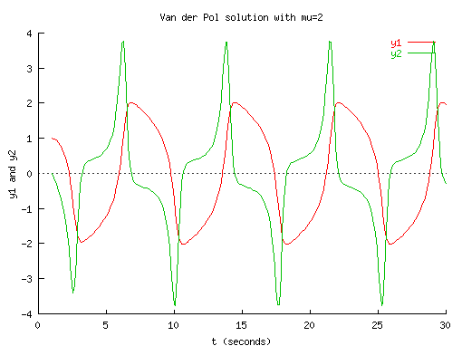
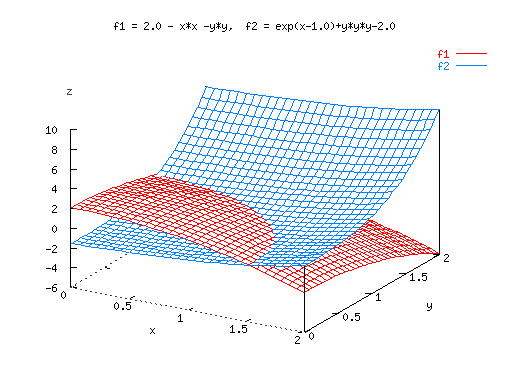
Sample screen shots of applications using numerical functions in Ch
are shown below. The source code for generating the graphical output
and more
Ch numerical computing
demos
are available. Using numerical computation features in Ch,
interactive numerical analysis
including
Web-based integration
and
ordinary differential equation solving
can be performed dynamically on-line.


|
|

